---

HiFrog demo presented in TACAS'17 is available here and another demo presented in SRI2021 summer school is available here.

How to run HiFrog for a specific theory of SMT?

HiFrog binary receives as input from the user a C-program with assertions to be verified, a set of parameters and the function summaries (either interpolation-based or user-defined) in the SMT-LIB Standard v. 2.0.

Throughout the example, note that the HiFrog environment should be prepared for analysis by cleaning the repository with $ rm __summaries before performing steps that do not use previous summaries. This is important especially when verifying a new benchmark, as the summaries of previously verified benchmarks must be removed.

HiFrog uses the CPROVER framework for pre-processing of C and translation to goto-program. All loops and a recursive function calls in the program should be unrolled using the command line --unwind <N>, where <N> is the number of loop iterations and the recursive depth. Any non-defined function is used to draw random values of an Integer, and any declared-only function is used to draw random values of a specific type (commonly denoted as nondet_int(), nondet_long(), etc.). The assumptions on the code for the verification process are given using __CPROVER_assume() notation, and thus, we can limit the values of non-deterministically chosen variables to a specific range or interval.

Basic Functionality of HiFrog

In this section, we explain how HiFrog constructs a function summary for an assertion (also referred to as to claim) and reuses it for another claim. The first example, shown in Fig. 1, consists of a function that randomly gets 1000 integers and returns their sum.

Use of Function summarization in verifying different assertions: In this example, we add assertions to the C-program that HiFrog verifies. The C-program with three assertions is shown in Fig. 1. Run HiFrog to check the first and the third assertion as follows:

$ rm __summaries
    $ ./hifrog --logic qflra ex1_lra.c --claim 1
    $ ./hifrog --logic qflra ex1_lra.c --claim 3

Figure 1: ex1_lra.c

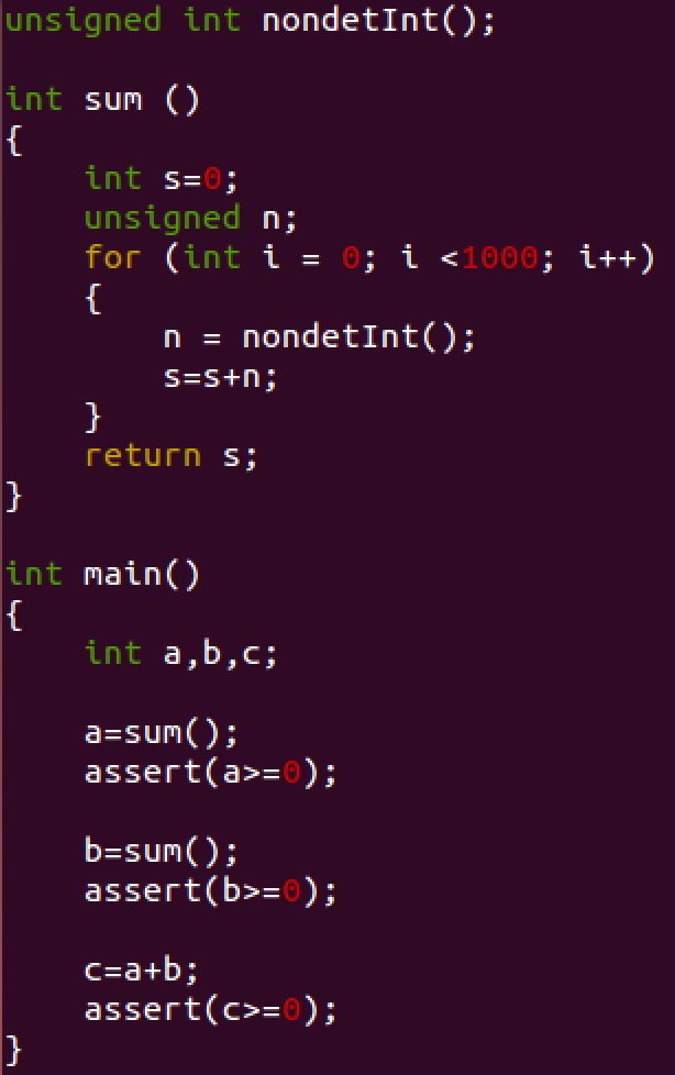
Note that summaries should not be removed after running the first claim.

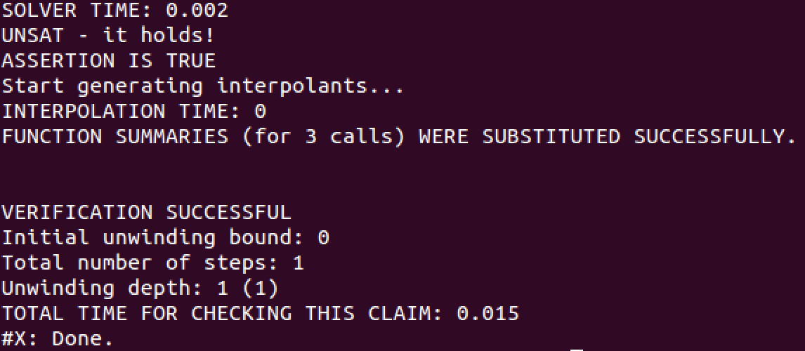
Fig. 2 and 3 show the relevant parts of the output from these two checks. On both figures, HiFrog indicates that the program is safe, reporting VERIFICATION SUCCESSFUL. Note that despite function nondetInt is declared-only, HiFrog is able to automatically identify its return type (unsigned int ) and exploit it for verification. We can also see the solver time and total time for checking these claims. The run time for the third claim is significantly lower than for the first claim due to summary usage.

Figure 2: Results of running HiFrog on ex1_lra.c (claim 1)

Figure 3: Results of running HiFrog on ex1_lra.c (claim 3)

What actually happened? When checking the second or third assertion HiFrog reuses the previous verification results for verifying the new claims. After the successful verification of the first assertion, HiFrog starts to generate the summaries which are stored for the subsequent verifications in the file __summaries. Since we specified the logic qflra, HiFrog generates the summaries in QF_LRA. We encourage the user to view the __summaries file. When checking the third assertion the generated summaries were substituted instead of encoding the function into the solver, and the speed-up we observe results from this. Since the verification of the third claim was successful, HiFrog updates the __summaries file with new function summaries.

Advanced Functionalities of HiFrog

HiFrog offers a number of interesting features that set it apart from many other model checkers. In the following, we describe the use of user-provided summaries, specification of different theories for modeling, automatica removal of some redundant assertions, and options for controlling the summary generation through interpolation.

User-Provided Summaries: HiFrog provides several approaches that can be used if the logic used for modeling is not sufficiently expressive. For example, this might happen when a user has non-linear arithmetics in the program. The LRA implementation of HiFrog will attempt to prove these properties by substituting the results of the unsupported operations with completely nondeterministic behavior to maintain soundness at the expense of providing spurious counter-examples, but sometimes this is not sufficient.

One way around this problem is to use the feature that allows the users to insert their own summaries for verification. These are provided in the SMT-LIB v2 format. To shed light on this issue, suppose that there is a C-code, shown in Fig. 4 which uses trigonometric functions and calculates Sinˆ2(x) + Cosˆ2(x). Since Sinˆ2(x) + Cosˆ2(x) = 1 for any x, as it is a known trigonometric identity, we can utilize this knowledge and substitute the formula with a summary stating exactly this identity.

Fig 4: sin_cos.c

To help the user get started with the summary construction we provide a command for constructing a summary template.

./hifrog --logic qflra --list-templates sin_cos.c

The above command dumps a list of templates for all functions used in the program into the summaries file. The following code snippet shows one of such the automatically generated templates that contains the define-fun statement, followed by the function name (nonlin ), the set of parameters, and the body of the function which is empty (it is indicated by true ).

Example of a summary template for nonlin function:

(define-fun |nonlin#0| ( 
        (|nonlin::x| Real) 
        (|hifrog::fun_start| Bool) 
        (|hifrog::fun_end| Bool)
        (|nonlin::#return_value| Real) ) Bool
        (let ( (?def0 true) )
            ?def0
        )
    )

Let's edit the template file by adding a new function summary which states that the return value of the function is 1, which is highlighted with pink in the following code snippet. Then save it in a file __summaries_nonlin

(define-fun |nonlin#0| ( (|nonlin::x| Real)
        (|hifrog::fun_start| Bool)
        (|hifrog::fun_end| Bool)
        (|nonlin::#return_value| Real) ) Bool
        (let ((?def0  (= 1 |nonlin::#return_value| )))
            ?def0
        )
    )

Now let's link the edited summary of nonlin function to the code sin_cos.c as follows.

$./hifrog --logic qflra sin_cos.c --load-summaries __summaries_nonlin

Intuitively, the use of user-defined summaries is to some extent similar to the use of user-defined assumptions. However, while assumptions just add additional constraints to the SMT formula and do not affect the encoding of the original code, our summaries are used to replace the code completely, thus (in program sin_cos.c) avoiding deal with complex nonlinear constraints.

Use of Uninterpreted Functions: Fig. 7 shows a function that multiplies two variables. Because of the non-linearity, LRA is not able to verify this program. Even though non-linear SMT solvers can verify such operations, it is usually costly and not supported by many solvers. The program could also be encoded using propositional logic, but due to the complicity of multiplication encoding this turns out to be expensive.

Fig. 7. ex1 uf.c

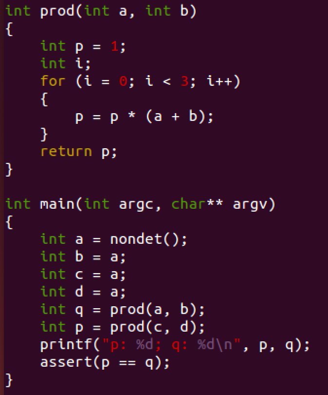
However, for this particular example, the correctness of the program does not depend on the exact interpretation of the multiplication. In fact, it suffices to assume that a function returns the same value when invoked with the same parameters. In the following, we verify the program specifying the logic QF_UF.

$ ./hifrog --claim 1 --logic qfuf ex1_uf.c

Use of Propositional Logic: In some cases, it is necessary to resort to the bit-precise modeling of the software through propositional logic despite the increased complexity this implies. This is supported in HiFrog currently through a separately built binary. For this particular example, the propositional logic check is done by running the following command:

$ ./hifrog --claim 1 --logic prop ex1_uf.c

 

In what follows, we outline various optimizations and unique features of HiFrog that can be useful in different stages of verification to simplify the life of users!

Removing redundant assertions: Fig. 8 shows a program calling a nondeterministic function sum1. Thus, the three assertions in the program are violated.

Fig. 8. ex2 lra.c

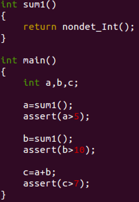
So the user can get a counter-example for each of them. Additionally, the user might be interested in running a dependency analysis to reveal other useful information about the assertions.

In particular, HiFrog has an option --claims-opt <steps> which identifies and reports the redundant assertions using the threshold <steps> as the maximum number of SSA steps between the assertions including the SSA steps at the functions calls (if any) between the assertions:

$ ./hifrog --logic qflra --claims-opt 20 ex2_lra.c

Fig. 9. Output for ex2_lra.c

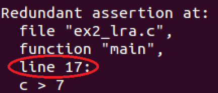
The expected result in Fig. 9 confirms the existence of the redundant assertion on line 17. Intuitively it means that the user should fix the other assertions first, and whenever it is done, the \redundant" assertion will hold automatically.

The approach we use for removing assertions is not complete in the sense that not all dependencies between assertions are detected. However, the process is sound in the sense that all dependencies are guaranteed to exist in the unwound version of the code.

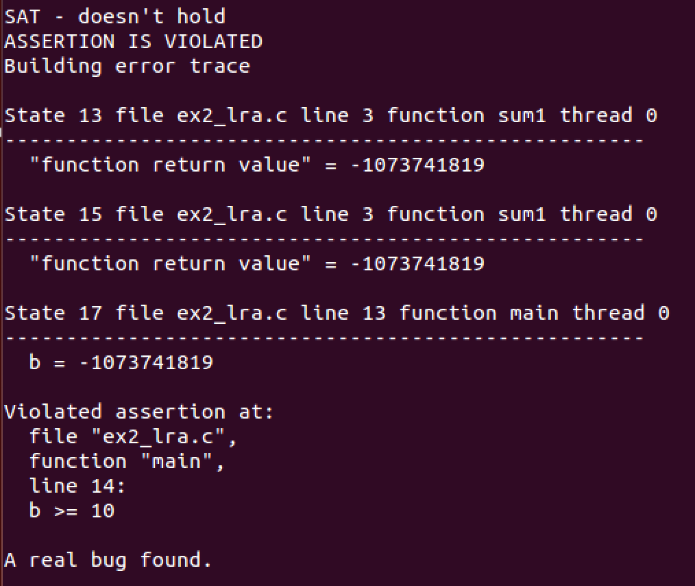
Error trace: Running HiFrog for the second assertion results in the output VERIFICATION FAILED and the corresponding error trace that manifests the bug.

Fig. 10. Counter example trace for ex2_lra.c

Tuning the Strength of Summaries: Interpolation can be tuned for strength by command line parameters for propositional logic, QF_LRA and QF_UF.

The parameter --itp-algorith <algo> specifies the interpolation algorithm for propositional logic, which is used for all theories. Variable <algo> ranges from 0 to 5, where the numerical values represent the propositional interpolation algorithms Ms, P, Mw, PS, PSw, PSs. The strength relation between the interpolation algorithms is such as Ms is the strongest, Mw is the weakest, PSs is stronger than PS and P, and PSw is weaker than P and PS. The specialized theory interpolation algorithms for QF_LRA and QF_UF can be specified, respectively, by --itp-lra-algorithm <algo> and --itp-uf-algorithm<algo>. As for LRA interpolation algorithms, the range of <algo> in --itp-lra-algorithm is as follows.

• 0 - Farkas_s 
• 2 - Dual Farkas
• 3 - Flexible Farkas (custom strength factor)
• 4 - Decomposing Farkas
• 5 - Dual Decomposing Farkas

For more details on LRA interpolation algorithms see here. As for UF interpolation algorithms, the range of <algo> in --itp-uf-algorithm is as follows.

• 0 - itp strong_s 
• 2 - itp weak
• 3 - itp random

For instance, verifying program uf_interpolation.c with the following command lines leads to summaries of different strength.

$ rm __summaries

$ ./hifrog --verbose-solver 2 --logic qfuf --itp-algorithm 0 --itp-uf-algorithm 0 --claim 1
     --save-summaries strong_summaries uf_interpolation.c

$ rm __summaries

$ ./hifrog --verbose-solver 2 --logic qfuf --itp-algorithm 0--itp-uf-algorithm 2 --claim 1
     --save-summaries weak_summaries uf_interpolation.c

Running HiFrog with the option --verbose-solver 2 enables printing of interpolants. Figures 11 and 12 show the interpolants generated for function mix (second interpolant printed by HiFrog), where the one generated with option 0 for --itp-uf-algorithm is strictly stronger than the one generated with option 2. These interpolants are used in the summary c::mix#0 in the les strong summaries and weak summaries.

Fig 11 Strong interpolant

Fig. 12. Weak interpolant

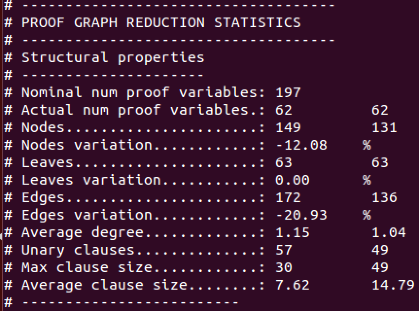
$ ./hifrog --verbose-solver 1 --reduce-proof --logic qfuf --itp-uf-algorithm 0 --claim 1 
    --save-summaries strong_summaries uf_interpolation.c

Fig. 13 shows a table from the log of HiFrog containing the effect of proof reduction. The first column lists different types of components of a proof, such as the number of variables, nodes and edges. The second column represents the corresponding statistics for the proof before reduction, and the third column for the proof after reduction. We can see in this example that the number of nodes was reduced from 149 to 131 (12.08%), and the number of edges was reduced from 172 to 136 (20.93%).

Fig. 13. Proof compression information